
Flexibly applying database functionality can easily achieve a 30,000-fold performance improvement in GIS selection scenarios.
| Level | Method | Performance/Time(ms) | Maintainability/Reliability | Notes |
|---|---|---|---|---|
| 1 | Brute Force | 30,000 | - | Simple form |
| 2 | Coordinate Index | 35 | Complexity/Magic Numbers | Extra complexity |
| 3 | Compound Index | 10 | Complexity/Magic Numbers | Extra complexity |
| 4 | GIST | 4 | Simplest expression, fully accurate | Simple form, more accurate distance, PostgreSQL specific |
| 5 | btree_gist Compound Index | 1 | Simplest expression, fully accurate | Simple form, more accurate distance, PostgreSQL specific |
Scenario#
Many internet businesses involve geography-related functional requirements, with nearest neighbor queries being the most common.
For example:
- Recommend nearby POIs (restaurants, gas stations, bus stops) to users
- Recommend nearby users (chat matching)
- Find addresses closest to user’s location (reverse geocoding)
- Find business districts, provinces, cities, districts, counties where users are located (point-to-polygon)
These problems are essentially nearest neighbor search or its variants.
Some functions seem unrelated to nearest neighbor search, but when you peel back the layers, they are also nearest neighbor search. A typical example is reverse geocoding:
When taking a ride-hailing service and selecting pickup locations, or when ordering food delivery and choosing delivery locations, the user’s current latitude/longitude coordinates are converted to textual geographic locations like “XX Community Building X”. This is actually a nearest neighbor search problem: find the coordinate point closest to the user’s current location.
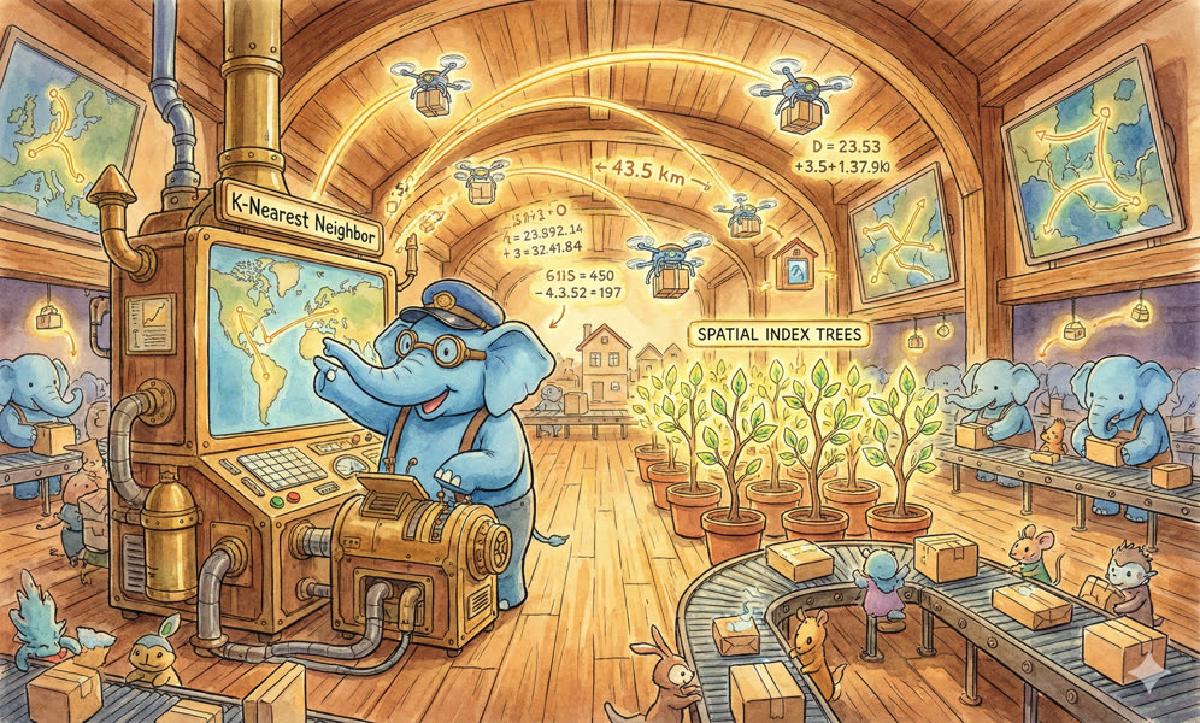
Nearest neighbor (KNN, k nearest neighbor), as the name suggests, is finding the K closest objects to a center point. The problem satisfies this form:
Find the closest K objects (and their attributes) that meet certain conditions.
Nearest neighbor search is such a commonly used function that optimization benefits are very significant.
Let’s start with a specific problem and describe the evolution of implementation methods for this functionality - how to achieve more than 30,000-fold performance improvement.
Problem#
We’ll choose recommending the nearest restaurants as a representative of this type of problem.
The problem is simple: Given a table pois containing all POI points in China and a latitude/longitude coordinate point, find the 10 restaurants closest to that coordinate point quickly enough. Return the names and distances of these ten restaurants.
Details:
The
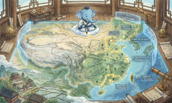
poistable contains 100 million records, of which POIs of restaurant type account for about 10 million.Given example center point: Beijing Normal University, 116.3660 E, 39.9615 N.
“Quickly enough” means completion within 1 millisecond
Distance means surface distance on Earth calculated in meters
poistable schema definition:CREATE TABLE pois ( id CHAR(10) PRIMARY KEY, name VARCHAR(100), position GEOMETRY, -- PostGIS ST_Point longitude FLOAT, -- Float64 latitude FLOAT, -- Float64 category INTEGER -- type of POI );Restaurant characteristic is
WHERE category BETWEEN 50000 AND 51000
Similar Problems#
This pattern applies to many examples. For Tantan (a dating app), it could be: find the 100 people closest to the user’s location, within a certain age range, plus some other filtering conditions.
For Meituan Dianping, it’s finding the 10 closest POIs of restaurant type to the user.
For reverse geocoding, it’s essentially finding the closest POI to the user (with optional type restrictions like intersections, landmark buildings, etc.)
Aside - Coordinate Systems: WGS84 and GCJ02
This is another area where many people get confused.
- Didi’s magical offset.
- Hong Kong, Macao, Taiwan borders, fragmented polygons.
Most internet geography-related functions involve nearest neighbor query requirements.
For dating scenarios, just replace WHERE category BETWEEN 50000 AND 51000 with WHERE age BETWEEN 18 AND 27.
Many students familiar with ACM competitions know various data structures and algorithms. They might be eager to try - R-tree, I choose you!
However, in real projects, data tables are data structures, and indexes with query methods are algorithms.
How is Distance Defined?#
To solve this problem, we need clear definitions. Distance definition is not as simple as it seems.
For example, for navigation software, distance might mean path length rather than straight-line distance.
In 2D plane coordinate systems, distance usually refers to Euclidean distance: $d=\sqrt{(x_2-x_1)^2+(y_2-y_1)^2}$
But in GIS, we usually use spherical coordinate systems, identifying points through latitude and longitude.
On a sphere, the distance between two points equals the arc length on the great circle of the sphere, which is the spherical angle × radius.
This introduces a problem: each degree of latitude corresponds to roughly constant distance, about 111 kilometers.
However, each degree of longitude corresponds to different distances depending on latitude. At the equator, it’s similar to latitude at about 111 kilometers, but as latitude increases, at 40° north latitude, one degree longitude corresponds to only 85 kilometers of arc length, and at the north pole, one degree longitude corresponds to 0 arc length distance.
In fact, there are other more complex problems. For example, Earth is actually an ellipsoid, not a perfect sphere.
Earth is not spherical, but an irregular ellipsoid. Initially, for simplicity, we can treat it as a sphere for distance calculations.
CREATE OR REPLACE FUNCTION sphere_distance(lon_a FLOAT, lat_a FLOAT, lon_b FLOAT, lat_b FLOAT)
  RETURNS FLOAT AS $$
SELECT asin(
           sqrt(
               sin(0.5 * radians(lat_b - lat_a)) ^ 2 +
               sin(0.5 * radians(lon_b - lon_a)) ^ 2 * cos(radians(lat_a)) * cos(radians(lat_b))
           )
       ) * 127561999.961088 AS distance;
$$
LANGUAGE SQL IMMUTABLE COST 100;
Using latitude/longitude coordinates as plane coordinates is not impossible, but for scenarios requiring precise sorting, such approximation may cause significant problems:
Each degree of longitude corresponds to different distances depending on latitude. At the equator, one degree longitude and latitude represent roughly the same distance of 111 kilometers, but as latitude increases, at 40° north latitude, one degree longitude corresponds to only 85 kilometers of arc length, and at the poles, one degree longitude corresponds to 0 arc length distance.
Therefore, a circle in plane coordinate system might only be a skinny ellipse in spherical coordinate system. When calculating distances, different distance weights in latitude and longitude directions can lead to serious correctness issues: a store 100 meters due north might rank higher in distance than one 70 meters due east. For high latitude regions, such problems become very serious.
Therefore, after brute force table scanning, precise distance calculation formulas usually need to be used again for calculation and sorting.
Note that the distance here has units not in meters but in degrees squared. Considering that 1 degree longitude and latitude correspond to vastly different actual distances in different places, this result has no precise practical meaning.
Latitude/longitude are spherical coordinates, not coordinates in 2D plane coordinate systems. However, for quick rough selection, this approach is acceptable.
For scenarios requiring precise sorting, spherical distance calculation formulas on Earth’s surface must be used, not simply calculating Euclidean distance.
How Fast is Fast Enough?#
In martial arts, nothing beats speed. The internet emphasizes speed - running fast, writing fast.
How fast is fast enough? One millisecond - that’s fast enough. This is also our optimization goal.
Alright, let’s get to the meat. Before PostGIS shows its true power, let’s first see how far traditional relational databases can go in solving this problem.
0x02 Solutions#
Let’s start with traditional relational databases
LEVEL-1 Brute Force Table Scan#
Using traditional relational databases, what solutions exist for this problem?
Brute force algorithms are very simple to write. Let’s take a look.
From the POIS table, first find all restaurants, get restaurant names, calculate distances from restaurants to our location, then sort by distance and take the closest 10 records.
A novice might quickly write such naive SQL:
SELECT
  id,
  name,
  sphere_distance(longitude, latitude,
                  116.3660 , 39.9615 ) AS d
FROM pois
WHERE category BETWEEN 50000 AND 51000
ORDER BY d
LIMIT 10;
To simplify the problem, let’s temporarily ignore the fact that latitude/longitude are actually spherical coordinates and Earth is an ellipsoid.
Under this assumption, this SQL can indeed complete the work correctly. However, anyone daring to use this in production would definitely get beaten up by the DBA.
Let’s first examine its execution plan:

Aside: SQL Inlining#
SQL inlining helps with correct index usage.
In real environments with fully warmed cache, actual execution time is 30 seconds; with PostgreSQL parallel query enabled (2 workers), actual execution time is 16 seconds.
Time: 30 seconds, actual execution time: 17 seconds.
Users are very sensitive to response time. When response time goes up, user satisfaction immediately drops. When playing King of Glory, even 100ms latency is very frustrating. If it’s a real-time application…
For tables with thousands of records, it might work adequately, but for tables with 100 million scale, brute force table scanning is not acceptable.
Users cannot accept waiting times of over ten seconds, let alone any scalability from such a design.
Existing Problems#
Outrageous Overhead#
This query needs to calculate distance between target point and all record points every time, then sort by distance and take TOP.
For tables with thousands of records, it might work adequately, but for tables with 100 million scale, brute force table scanning is not acceptable. Users cannot accept waiting times of over ten seconds, let alone any scalability.
Questionable Correctness#
Using latitude/longitude coordinates as plane coordinates is not impossible, but for scenarios requiring precise sorting, such approximation may cause significant problems:
Each degree of longitude corresponds to different distances depending on latitude. At the equator, one degree longitude and latitude represent roughly the same distance of 111 kilometers, but as latitude increases, at 40° north latitude, one degree longitude corresponds to only 85 kilometers of arc length, and at poles, one degree longitude corresponds to 0 arc length distance.
Therefore, a circle in plane coordinate system might only be a skinny ellipse in spherical coordinate system. When calculating distances, different distance weights in latitude and longitude directions can lead to serious correctness issues: a store 100 meters due north might rank higher than one 70 meters due east. For high latitude regions, such problems become very serious.
Therefore, after brute force table scanning, precise distance calculation formulas usually need to be used again for calculation and sorting.
Aside: Incorrect Index Usage is Counterproductive#
Some might say the POI type field category appears in the query’s WHERE condition and can be improved through indexing.
This time instead of direct table scanning, it first scans the index on category, filtering out all restaurant records.
Then it scans page by page according to the index.
Result: sequential IO becomes random IO.
So what’s the correct way to use indexes?
LEVEL-2 Coordinate Indexes#
Indexes are the bread and butter of relational databases. Since sequential table scanning is not acceptable, we naturally think of using indexes to accelerate queries.
The naive approach is to filter candidate points within a certain range around the target point through indexes, then further calculate distances and sort.
Using indexes on latitude/longitude is based on this idea:
Beijing Normal University is in the prosperous center of the universe in the capital. If we draw a square with 1km sides (or a circle with 1km diameter) on the map, not to mention 10 restaurants - even 100 might be possible.
Conversely, since the closest 10 restaurants must fall within such a large circle, and this table’s POI points include POI points from all of China, filter candidate points within a certain range around the target point, then further calculate distances and sort.
CREATE INDEX ON pois1 USING btree(longitude);
CREATE INDEX ON pois1 USING btree(latitude);
Also, to solve the correctness problem, assume we have a SQL function sphere_distance that calculates spherical distance from latitude/longitude:
CREATE FUNCTION sphere_distance(lon_a FLOAT, lat_a FLOAT, lon_b FLOAT, lat_b FLOAT) RETURNS FLOAT
IMMUTABLE LANGUAGE SQL COST 100 AS $$
SELECT asin(
           sqrt(
               sin(0.5 * radians(lat_b - lat_a)) ^ 2 +
               sin(0.5 * radians(lon_b - lon_a)) ^ 2 * cos(radians(lat_a)) *
               cos(radians(lat_b))
           )
       ) * 127561999.961088 AS distance;
$$;
So if using a 1km-sided square centered on the target point for initial screening, this query can be written as:
SELECT
  id, name,
  sphere_distance(longitude, latitude, 116.365798, 39.966956) as d
FROM pois1
WHERE
  longitude BETWEEN 116.365798 - 0.5 / 85 AND 116.365798 + 0.5 / 85 AND
  latitude BETWEEN 39.966956 - 0.5 / 111 AND 39.966956 + 0.5 / 111  AND
  category = 60000
ORDER BY 3 LIMIT 10;
After warming up, actual execution averages 35 milliseconds - nearly 1000x performance improvement over brute force table scanning, a huge progress.

For relatively simple rough products, this method has reached ‘usable’ levels. But this method still has many problems.
Existing Problems#
The biggest problem with this method is additional complexity. It uses one (or multiple) magic numbers to determine the rough range of candidate points.
The selection of this magic number relies on our prior knowledge. We clearly know that with the commercial density of the prosperous cosmic center Wudaokou, there are definitely more than 10 shops within a 1km square. But for extreme scenarios (which might actually be common), like in the Taklamakan Desert or Qiangtang No-man’s Land, the nearest shop logically must exist, but its distance might exceed several hundred kilometers.
This method’s performance is extremely sensitive to magic number selection: choosing too large a distance causes performance to deteriorate rapidly; choosing too small a distance might return no results for remote countryside areas. Programmers have one more headache.
Time: 35 milliseconds
1000x improvement - not bad, but don’t celebrate too early.
What do all these strange constants mean?
1000x performance improvement - let’s look at the query execution plan to see how it’s achieved.
First, on longitude, it uses index scanning to generate a bitmap.
Then, on latitude, it also uses index scanning to generate another bitmap.
Next, the two bitmaps perform bitwise operations to generate a new bitmap, filtering records that meet latitude/longitude conditions.
Then it scans these qualifying candidate points, calculates distances, and sorts.
We chose boundary values quite cleverly, so records actually participating in distance calculation and sorting might only be around 30.
Compared to the previous 10+ million distance calculations and sorting, this is obviously much more sophisticated.
Aside: Hyperparameters and Additional Complexity#
Because this boundary magic number is well-chosen, performance is relatively ideal.
The biggest problem with this method is additional complexity. It uses one (or multiple) magic numbers to determine the rough range of candidate points.
The selection of this magic number relies on our prior knowledge. We clearly know that with the commercial density of the prosperous cosmic center Wudaokou, there are definitely more than 10 shops within a 1km square. But for extreme scenarios (which might actually be common), like in the Taklamakan Desert or Qiangtang No-man’s Land, the nearest shop logically must exist, but its distance might exceed several hundred kilometers.
This method’s performance is extremely sensitive to magic number selection: choosing too large a distance causes performance to deteriorate rapidly; choosing too small a distance might return no results for remote countryside areas. Programmers have one more headache.
Let’s ignore this annoying problem for now and see if traditional relational databases can be squeezed further.
Bad Cases#
Because this boundary magic number is well-chosen, performance is relatively ideal.
The biggest problem with this method is additional complexity. It uses one (or multiple) magic numbers to determine the rough range of candidate points.
The selection of this magic number relies on our prior knowledge. We clearly know that with the commercial density of the prosperous cosmic center Wudaokou, there are definitely more than 10 shops within a 1km square. But for extreme scenarios (which might actually be common), like in the Taklamakan Desert or Qiangtang No-man’s Land, the nearest shop logically must exist, but its distance might exceed several hundred kilometers.
This method’s performance is extremely sensitive to magic number selection: choosing too large a distance causes performance to deteriorate rapidly; choosing too small a distance might return no results for remote countryside areas. Programmers have one more headache.
Let’s ignore this annoying problem for now and see if traditional relational databases can be squeezed further.
| Large Radius Poor Performance | Small Radius Can’t Circle Enough |
|---|---|
 | 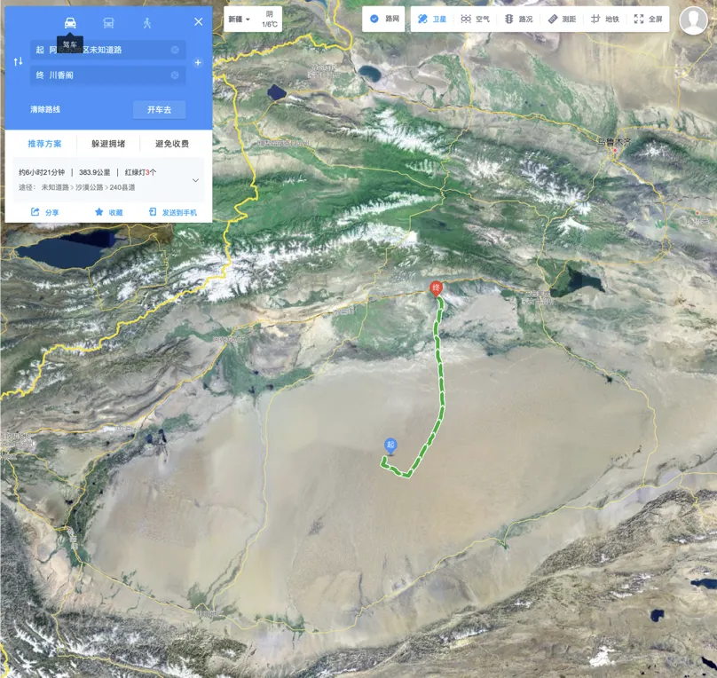 |
| Prosperous Wudaokou, 10 shops in 1km easy. | 300km away for one shop, Xinjiang people cry in toilets |
LEVEL-3 Compound Index and Clustering#
Putting aside the troubles caused by magic numbers, let’s study how far traditional relational databases can go in solving this problem.
Replace individual indexes on each column with multi-column indexes and cluster the table by that index.
Still the exact same query statement
Improved from 30ms to 10ms, 3x performance improvement
For traditional relational databases, this is about the limit
Is there an elegant, correct, fast solution?

CREATE INDEX ON pois4 USING btree(longitude, latitude, category);
CLUSTER pois4 USING pois4_longitude_latitude_category_idx;
The corresponding query remains unchanged:
SELECT id, name,
	sphere_distance(longitude, latitude, 116.365798, 39.966956) as d FROM pois4
WHERE
  longitude BETWEEN 116.365798 - 0.5 / 85  AND 116.365798 + 0.5 / 85  AND
  latitude  BETWEEN  39.966956 - 0.5 / 111 AND 39.966956  + 0.5 / 111 AND
  category = 60000
ORDER BY sphere_distance(longitude, latitude, 116.365798, 39.966956)
LIMIT 10;
Compound index query execution plan can compress actual execution time to 7 milliseconds.

This is about the limit for traditional relational data models. For most businesses, this is an acceptable level.
Because this boundary magic number is well-chosen, performance is relatively ideal.
Extension Variant: GeoHash#
GeoHash is a variant of this approach. By encoding 2D latitude/longitude into 1D strings, traditional string prefix matching operations can be used to filter geographic locations. However, fixed granularity significantly reduces flexibility. Whether to use compound indexes or special encoded redundant fields needs analysis for specific scenarios.
Still the exact same query statement
Improved from 30ms to 10ms, 3x performance improvement
For traditional relational databases, this is about the limit
Is there an elegant, correct, fast solution?
LEVEL-4 GIST#
Is there a way to complete this work elegantly, efficiently, and concisely?
PostGIS provides an excellent solution: switch to Geometry type and create GIST indexes.
CREATE TABLE pois5(
  id       CHAR(10) PRIMARY KEY,
  name     VARCHAR(100),
  position GEOGRAPHY(Point), -- PostGIS ST_Point
  category INTEGER   -- type of POI
);

CREATE INDEX ON pois5 USING GIST(position);
SELECT id, name FROM pois6 WHERE category = 60000
ORDER BY position <-> ST_GeogFromText('SRID=4326;POINT(116.365798 39.961576)') LIMIT 10;R-tree#
The core idea of R-tree is to aggregate closely distant nodes and represent them as minimum bounding rectangles of these nodes at the upper layer of the tree structure. This minimum bounding rectangle becomes a node at the upper layer. Because all nodes are within their minimum bounding rectangles, queries that don’t intersect with a rectangle definitely don’t intersect with all nodes in that rectangle.

In actual queries, this query can complete in 1.6 milliseconds - quite an amazing result. But note that position here is of type GEOMETRY, meaning it uses 2D plane coordinates. Correct distance calculation requires using Geography type.
SELECT
  id,
  name,
  position <->
  ST_Point(116.3660, 39.9615)::GEOGRAPHY AS d
FROM pois5
WHERE category BETWEEN 50000 AND 51000
ORDER BY d
LIMIT 10;
Because spherical distance calculations cost much more than plane distance, using Geography to replace Geometry incurs overhead - about 4.5ms.
One-fold performance loss is quite considerable, so in daily applications, you need to carefully balance precision and performance.
Usually topological queries and rough people-circling are suitable for Geometry type, while precise calculations and judgments must use Geography type. Here, sorting by distance requires precise distance, so Geography is used.
| Geometry: 1.6 ms | Geography: 3.4 ms |
|---|---|
 |  |
Now let’s see PostGIS’s answer.
PostGIS uses different data types, indexes, and query methods.
First, the data type here is no longer two floating-point numbers but becomes a Geography field containing a pair of latitude/longitude coordinates.
Then, the index we use is no longer the common Btree index but GIST index.
Generalized Search Tree - a universal search tree with balanced tree structure. For spatial geometric types, the implementation usually uses R-tree.
Usually topological queries and rough people-circling are suitable for Geometry type, while precise calculations and judgments must use Geography type. Here, sorting by distance requires precise distance, so Geography is used.
Aside: Geometry or Geography?#
Because spherical distance calculations cost much more than plane distance, using Geography to replace Geometry incurs overhead
Topological relationships and rough estimates use Geometry; precise calculations use Geography
Computational overhead is about one-fold; need to carefully balance correctness/precision and performance.
Now let’s see PostGIS’s answer.
PostGIS uses different data types, indexes, and query methods.
First, the data type here is no longer two floating-point numbers but becomes a Geography field containing a pair of latitude/longitude coordinates.
Then, the index we use is no longer the common Btree index but GIST index.
Generalized Search Tree - a universal search tree with balanced tree structure. For spatial geometric types, the implementation usually uses R-tree.
Usually topological queries and rough people-circling are suitable for Geometry type, while precise calculations and judgments must use Geography type. Here, sorting by distance requires precise distance, so Geography is used.
LEVEL-5 btree_gist#
Can we go further?
Observing the execution plan in Level-4, we find the condition on category doesn’t use indexes.
Can we create a compound index of position and category like the optimization in Level-3?
Unfortunately, B-tree and R-tree are two completely different data structures with different usage methods.
So we have this idea: can we treat category as the third dimension coordinate of position, letting R-tree directly index in 3D space?
This idea is correct, but it doesn’t need to be so complicated.
One problem with GIST indexes is that they work differently from B-trees and cannot create GIST indexes on data types that don’t support GIST index methods.
Usually, geometric types and range types support GIST indexes, but strings, numeric types, etc. don’t support GIST. This makes it impossible to create multi-column indexes like GIST(position, category).
PostgreSQL’s built-in btree_gist extension solves this problem.
PostgreSQL’s built-in extension btree_gist allows creating compound indexes of regular types and geometric types.
CREATE EXTENSION btree_gist;

CREATE INDEX ON pois6 USING GIST(position, category);

CLUSTER VERBOSE pois6 USING idx_pois6_position_category_gist;
The same query can be simplified to:
SELECT id, name, position <-> ST_Point(lon, lat) :: GEOGRAPHY AS distance
FROM pois6 WHERE category = 60000 ORDER BY 3 LIMIT 10;| Geometry: 0.85ms / Geography: 1.2ms |
|---|
 |
CREATE OR REPLACE FUNCTION get_random_nearby_store() RETURNS TEXT
AS $$
DECLARE
  lon FLOAT := 110 + (random() - 0.5) * 10;
  lat FLOAT := 30 + (random() - 0.5) * 10;
BEGIN
  RETURN (
    SELECT jsonb_pretty(jsonb_build_object('list', a.list, 'lon', lon, 'lat', lat)) :: TEXT
    FROM (
           SELECT json_agg(row_to_json(top10)) AS list
           FROM (
             SELECT id, name, position <-> ST_Point(lon, lat) :: GEOGRAPHY AS distance
             FROM pois6 WHERE category = 60000 ORDER BY 3 LIMIT 10 ) top10
         ) a);
END;
$$ LANGUAGE PlPgSQL;
import http, http.server, random, psycopg2
class GetHandler(http.server.BaseHTTPRequestHandler):
conn = psycopg2.connect("postgres://localhost:5432/geo")
def do_GET(self):
self.send_response(http.HTTPStatus.OK)
self.send_header('Content-type','application/json')
with GetHandler.conn.cursor() as cursor:
cursor.execute('SELECT get_random_nearby_store() as res;')
res = cursor.fetchone()[0]
self.wfile.write(res.encode('utf-8'))
return
with http.server.HTTPServer(("localhost", 3001), GetHandler) as httpd: httpd.serve_forever()Case Summary#
| Level | Method | Performance/Time(ms) | Maintainability/Reliability | Notes |
|---|---|---|---|---|
| 1 | Brute Force | 30,000 | - | Simple form |
| 2 | Coordinate Index | 35 | Complexity/Magic Numbers | Extra complexity |
| 3 | Compound Index | 10 | Complexity/Magic Numbers | Extra complexity |
| 4 | GIST | 4 | Simplest expression, fully accurate | Simple form, more accurate distance, PostgreSQL specific |
| 5 | btree_gist Compound Index | 1 | Simplest expression, fully accurate | Simple form, more accurate distance, PostgreSQL specific |
Well then, after this long journey, through PostGIS and PostgreSQL, we’ve accelerated a query that originally took 30,000 milliseconds to 1 millisecond - a 30,000-fold improvement. Compared to traditional relational databases, besides more than 10x performance improvement, there are many other advantages:
The SQL form is very simple - just the brute force table scan SQL without any strange additional complexity. And distance calculations use more precise WGS84 ellipsoid spherical distances.
So what conclusions can we draw from this example? PostGIS’s performance is excellent. How does it perform in actual production environments?
We can replace the position here from restaurant locations to user locations, and replace POI category ranges with candidate age ranges. This is the scenario faced by Tantan’s matching functionality.
Performance in Real Scenarios#
Performance is important. In martial arts, nothing beats speed.
Currently, the database uses a total of 220 machines with business QPS near 100,000. Database TPS peaks at around 2.5 million. The core database has a 1-master-19-slave configuration.
Our company’s SLA for databases is: 99.99% of regular database requests need to complete within 1 millisecond, while single database node QPS peaks around 30,000. These two are closely related - if a request can complete in 1 millisecond, then for a single thread, 1000 requests can be processed per second. Our database physical machines have 24-core 48-thread CPUs, but hyperthreaded machine CPU utilization is around 60%-70%. This roughly translates to 30 usable cores. So the QPS that all cores can handle is 30*1000=30,000. At an 80% CPU limit water level, the QPS ceiling is around 38k, which matches real stress test results.
Compiled from my presentation at the 2018 Hieroglyphic China Beijing PostGIS Special Session. Please retain source when reposting.