
Information theory answers two fundamental questions in communication theory:
- The critical value for data compression: entropy \(H\)
- The critical value for communication transmission rate: channel capacity \(C\)
But information theory’s content extends far beyond this—we encounter it in many fields: communication theory, computer science, physics (thermodynamics), probability theory and statistics, philosophy of science, economics, and more.
Entropy#
Information is a rather broad concept that’s difficult to capture completely and accurately with a simple definition. However, for any probability distribution, we can define a quantity called entropy that possesses many properties intuitively required for measuring information.
Entropy is a measure of the uncertainty of random variables, and also a measure of the information needed to describe random variables on average.
Let \(X\) be a discrete random variable with alphabet \(\mathcal{X}\). The probability density function \(p(x) \equiv Pr(X=x),x\in \mathcal{X}\) is denoted as \(p(x)\). Then:
Definition: Entropy#
The entropy $H(X)$ of a discrete random variable $X$ is defined as:
$$ H(X) = - \sum_{x \in \mathcal{X}}{p(x)\log_2{p(x)}} $$Since $x\log(x) → 0$ as $x → 0$, but $\log x$ is undefined at zero, we adopt the convention $0\log0 = 0$.
Sometimes the above quantity is denoted as $H(p)$. When using logarithms with base 2, entropy is measured in bits. When using natural logarithms with base $e$, entropy is measured in nats.
Since $p(x)$ is the probability distribution function of $X$, entropy can alternatively be viewed as the expected value of the random variable $\log{\frac{1}{p(X)}}$, denoted as $-E\log p(X)$.
Properties#
- $H(X) \ge 0$: Entropy is non-negative, because probability $0 \le p(x) \le 1$, so $\log\frac 1 {p(x)} ≥ 0$.
- $H_b(X) = (\log_b a) H_a(X)$: Base conversion for entropy, because $\log_b p = (\log_b a)\log_a p$, so $\ln(p) = \ln(a) H(X)$.
Example#
For a single Bernoulli trial with success probability $p$, if the random variable of the experimental result is $X$, its entropy is:
$$ H(X) = - [ p\log p + (1-p)\log (1-p)] $$When $p = \frac 1 2$, the entropy of the resulting random variable $X$ is: 1 bit.
Intuition#
Although the definition of entropy can be derived from several properties we require, there’s actually profound intuition behind this definition. For example:
We need to design binary encoding for an alphabet to minimize average information length. Letters often appear with unequal probabilities, so we need to follow the principle of higher frequency letters get shorter codes. Optimal encoding requires assigning appropriate costs to each letter to minimize total average cost. What constitutes an appropriate cost? A simple, intuitive principle is: the encoding cost of each letter should be proportional to its occurrence probability $p(x)$.

On the other hand, we need to consider the relationship between optimal encoding length $L(x)$ and encoding cost for letter $x$. Variable-length encoding has a problem: to ensure every message string can be unambiguously segmented and decoded, no word’s code can be a prefix of another word’s code, otherwise conflicts arise. For binary encoding, we can use 0 as a terminating delimiter. Thus, for four words A, B, C, D, they can be encoded as 0, 10, 110, 111 respectively. For each letter, when assigned an encoding of length $L=l$, what’s the cost? In the entire encoding space, all codes with this letter’s encoding as prefix can no longer be assigned. For example, after assigning B the 2-bit code 10, all codes like 100, 101, 1000, 1001, ... become unavailable—one-quarter of the entire encoding space is lost as cost.
So for a binary message with encoding length $L$, its cost is $\frac 1 {2^L}$, i.e., $cost = \frac 1 {2^L}$. Conversely, for letter $x$ with occurrence probability $p(x)$, the optimal encoding length should be:
$$ L(x) = \log_2 {\frac 1 {cost}} = \log_2 {\frac 1 {p(x)}} $$Then it becomes clear: the optimal encoding length $L$ for letter $x$, weighted by its occurrence probability $p(x)$, gives the optimal average encoding length—which is entropy!
$$ \sum_{x \in \mathcal{X}} {p(x)L(x)} = \sum_{x \in \mathcal{X}} {p(x)\log_2{\frac 1 {p(x)}}} = \sum_{x \in \mathcal{X}} -p(x)\log_2 p(x) = H(X) $$Joint Entropy#
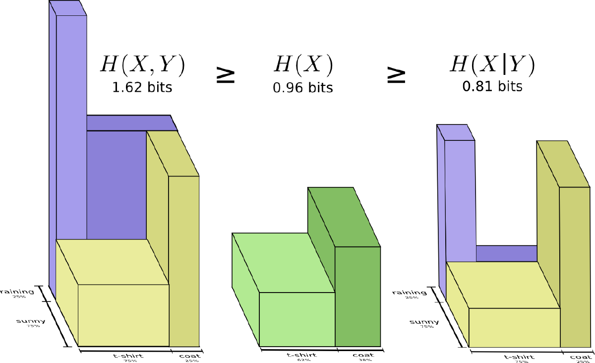
Extending the entropy of a single random variable to two random variables gives us the concept of joint entropy.
Definition: Joint Entropy#
For a pair of discrete random variables $(X,Y)$ with joint probability distribution $p(x,y)$, their joint entropy $H(X,Y)$ is defined as:
$$ H(X,Y) = - \sum_{x \in \mathcal{X}} \sum_{y \in \mathcal{Y}} p(x,y)\log p(x,y) $$Abbreviated as:
$$ H(X,Y) = -E\log p(X,Y) $$
Conditional Entropy#
The entropy of one random variable given another random variable is called conditional entropy.
Definition: Conditional Entropy#
If $(X,Y) \sim p(x,y)$, conditional entropy $H(Y|X)$ is defined as:
$$ H(Y|X) = \sum_{x \in \mathcal{X}}p(x)\ H(Y | X = x) = -E\log p(Y | X) $$Property#
$$ H(X,Y) = H(X) + H(Y|X) $$
Mutual Information#
Consider two random variables $X,Y$ with joint probability density function $p(x,y)$ and marginal probability density functions $p(x), p(y)$ respectively. Mutual information $I(X;Y)$ is defined as the relative entropy between their joint distribution $p(x,y)$ and product distribution $p(x)p(y)$:
$$ I(X;Y) = \sum_{x\in \mathcal{X}} \sum_{y \in \mathcal{Y}} {p(x,y)\log \frac{p(x,y)}{p(x)\ p(y)}} = D( p(x,y)\ \|\ p(x)\ p(y)) $$Expressing mutual information as the relative entropy between joint distribution and product of distributions measures how independent the two random variables $X,Y$ are.
As an extreme case, when $X=Y$, the two random variables are perfectly correlated, and $I(X;X)=H(X)$. Therefore, entropy is sometimes called self-information.
| Independent Variables | Non-independent Variables |
|---|---|
 |  |
Of course, mutual information can actually be expressed in another more intuitive way. If random variables $X,Y$ have entropies $H(X), H(Y)$ and joint entropy $H(X,Y)$, then mutual information can be expressed as:
$$ I(X;Y) = H(X) + H(Y) - H(X,Y) $$This is easily understood, because $H(X)+H(Y)$ contains two copies of shared information, while $H(X,Y)$ contains only one.
Property#
For any two random variables $X,Y$:
$$ I(X;Y) \ge 0 $$with equality if and only if $X,Y$ are mutually independent.
This shows that knowing any other random variable $Y$ can only reduce the uncertainty of $X$.
Relationships among Mutual Information I(X;Y), Self-information H(X), Joint Information H(X,Y), Conditional Information H(Y|X)#
A single diagram illustrates all relationships:


Cross Entropy and Relative Entropy#
For a random distribution $p$, if we use encoding $L=-log,p(x)$ optimized for distribution $p$, the average message length is:
$$ H(p) = - \sum_{x}{p(x)\log {p(x)}} $$In this case, it can be proven that average encoding length is optimal. But if we use encoding $L = -log,q(x)$ optimized for another random distribution $q$, some inefficiency occurs. The average message length then requires $H_q(p)$ bits:
$$ H_q(p) =- \sum_{x} p(x)\log q(x) $$Here the actual distribution is $p$, but the cost $-log,q(x)$ assigned to letter $x$ is optimized according to distribution $q$.
$H_q(p)$ is called the cross entropy of distribution $p$ relative to distribution $q$.
The cross entropy of $p$ with respect to $q$ can be decomposed into the sum of two parts: the entropy $H(p)$ of distribution $p$ itself, and the relative entropy $D(p | q)$ of $p$ relative to $q$:
$$ H_q(p) = H(p) + D(p \| q) $$
Relative entropy $D$, also known as Kullback-Leibler divergence (KLD), information divergence, information gain, or KL distance, is a measure of distance between two random distributions. Relative entropy $D(p |q)$ measures the inefficiency when the true distribution is $p$ but we assume distribution $q$.
Definition: Relative Entropy#
The relative entropy between two probability density functions $p(x)$ and $q(x)$ is defined as:
$$ D(p \| q) = \sum_{x \in \mathcal{X}}{p(x)\log \frac{p(x)}{q(x)}} = E_p\log \frac{p(X)}{q(X)} $$Properties#
- Relative entropy is always non-negative. When $p=q$, the optimal encoding for $q$ is also optimal for $p$, so $D(p | q) = 0$.
- Relative entropy is not symmetric: $D(p|q) \ne D(q|p)$.
Applications#
Cross entropy, as a measure of difference between two distributions, is widely used in machine learning. For example, when used as a neural network cost function:
$$ C = - [ y\ln(y') + (1-y)\ln(1-y')] $$where $y$ is the sample label, serving as the reference distribution $q(x)$, and $y’$ is the neural network’s inference output, serving as the actual working result distribution $p(x)$.